numpy&pandas基础
numpy基础
1 | import numpy as np |
定义array
1 2 3 4 5 6 7 8 9 10 11 12 13 14 15 16 17 18 19 20 21 22 23 24 25 26 27 28 29 30 31 32 33 34 35 36 37 38 39 40 41 42 43 44 45 46 47 48 49 50 51 52 53 54 | In [156]: np.ones(3)Out[156]: array([1., 1., 1.])In [157]: np.ones((3,5))Out[157]: array([[1., 1., 1., 1., 1.], [1., 1., 1., 1., 1.], [1., 1., 1., 1., 1.]])In [158]: In [158]: np.zeros(4)Out[158]: array([0., 0., 0., 0.])In [159]: np.zeros((2,5))Out[159]: array([[0., 0., 0., 0., 0.], [0., 0., 0., 0., 0.]])In [160]: In [146]: a = np.array([[1,3,5,2],[4,2,6,1]])In [147]: print(a)[[1 3 5 2] [4 2 6 1]]In [148]:In [161]: np.arange(10)Out[161]: array([0, 1, 2, 3, 4, 5, 6, 7, 8, 9])In [162]: np.arange(3,13)Out[162]: array([ 3, 4, 5, 6, 7, 8, 9, 10, 11, 12])In [163]: np.arange(3,13).reshape((2,5))Out[163]: array([[ 3, 4, 5, 6, 7], [ 8, 9, 10, 11, 12]])In [164]: In [169]: np.arange(2,25,2)Out[169]: array([ 2, 4, 6, 8, 10, 12, 14, 16, 18, 20, 22, 24])In [170]: np.arange(2,25,2).reshape(3,4)Out[170]: array([[ 2, 4, 6, 8], [10, 12, 14, 16], [18, 20, 22, 24]])In [171]: In [176]: np.linspace(1,10,4)Out[176]: array([ 1., 4., 7., 10.])In [177]: |
array基本运算
1 2 3 4 5 6 7 8 9 10 11 12 13 14 15 16 17 18 19 20 21 22 23 24 25 26 27 28 29 30 31 32 33 34 35 36 37 38 39 40 41 42 43 44 45 46 47 48 49 50 51 52 53 54 55 56 57 58 59 60 61 62 63 64 65 66 67 68 69 70 71 72 73 74 75 76 77 78 79 80 81 82 83 84 85 86 87 88 89 90 91 92 93 94 95 96 97 98 99 100 101 102 103 104 105 106 107 108 109 110 111 112 113 114 115 116 117 118 119 120 121 122 123 124 125 126 127 128 129 130 131 132 133 134 135 136 137 138 139 140 141 142 143 144 145 146 147 148 149 150 151 152 153 154 155 156 157 158 159 160 161 162 163 164 165 166 167 168 169 170 171 172 173 174 175 176 177 178 179 180 181 182 183 184 185 186 187 188 189 190 191 192 193 194 195 196 197 198 199 200 201 202 203 204 205 206 207 208 209 210 211 212 213 214 215 216 217 218 219 220 221 222 223 224 225 226 227 228 229 230 231 232 233 234 235 236 237 238 239 240 241 242 243 244 245 246 247 248 249 250 251 252 253 254 255 256 257 258 259 260 261 262 263 264 265 266 267 268 269 270 271 272 273 274 275 276 277 278 279 280 281 282 283 284 285 286 287 288 289 290 291 292 293 294 295 296 297 298 299 300 301 302 303 304 305 306 307 308 309 310 311 312 313 314 315 316 317 318 319 320 321 322 323 324 325 326 327 328 329 330 331 332 333 334 335 336 337 338 339 340 341 342 343 344 | In [7]: a = np.array([[1,2],[3,4]])In [8]: b = np.arange(5,9).reshape((2,3))In [10]: print(a)[[1 2] [3 4]]In [11]: print(b)[[5 6] [7 8]]In [12]:In [12]: a+bOut[12]: array([[ 6, 8], [10, 12]])In [13]: a-bOut[13]: array([[-4, -4], [-4, -4]])In [14]: a*b # 对应元素相乘Out[14]: array([[ 5, 12], [21, 32]])In [17]: a/bOut[17]: array([[0, 0], [0, 0]])In [18]: In [18]: a**2Out[18]: array([[ 1, 4],[ 9, 16]])In [19]:In [15]: np.dot(a,b) # 矩阵乘法Out[15]: array([[19, 22],[43, 50]])In [16]: a.dot(b)Out[16]: array([[19, 22],[43, 50]])In [17]:In [54]: print(a)[[ 2 3 4 5] [ 6 7 8 9] [10 11 12 13]]In [55]: np.sum(a)Out[55]: 90In [56]: np.min(a)Out[56]: 2In [57]: np.max(a)Out[57]: 13In [58]: In [58]: np.sum(a,axis=1)Out[58]: array([14, 30, 46])In [59]: np.sum(a,axis=0)Out[59]: array([18, 21, 24, 27])In [60]:# 三角函数结合random生成一组随机数据In [74]: N = 10In [75]: t = np.linspace(0, 2*np.pi, N)In [76]: print(t)[0. 0.6981317 1.3962634 2.0943951 2.7925268 3.4906585 4.1887902 4.88692191 5.58505361 6.28318531]In [77]: y = np.sin(t) + 0.02*np.random.randn(N)In [78]: print(y)[-0.00947902 0.64196198 0.96567468 0.89394571 0.33830193 -0.3015316 -0.86943758 -0.95954123 -0.62526393 0.02872202]In [79]: M = 3 In [80]: for ii, vv in zip(np.random.rand(M)*N, np.random.randn(M)): ...: y[int(ii):] += vv ...: In [81]: print(y)[-0.00947902 0.64196198 1.47685437 1.55309848 0.99745469 0.35762117 -0.21028481 -0.30038846 -0.29746375 0.35652221]In [82]: In [101]: a = np.arange(2,14).reshape((3,4)) In [102]: print(a)[[ 2 3 4 5] [ 6 7 8 9] [10 11 12 13]]In [103]: print(np.argmin(a)) # 最小值的索引0In [104]: print(np.argmax(a)) # 最大值的索引11In [105]: np.cumsum(a) # 从0元素开始的累计和Out[105]: array([ 2, 5, 9, 14, 20, 27, 35, 44, 54, 65, 77, 90])In [106]: np.cumprod(a) # 从1元素开始的累计乘Out[106]: array([ 2, 6, 24, 120, 720, 5040, 40320, 362880, 3628800, 39916800, 479001600, 6227020800])In [107]: In [129]: aOut[129]: array([[ 2, 3, 4, 5], [ 6, 7, 8, 9], [10, 11, 12, 13]])In [130]: np.cumsum(a,axis=1)Out[130]: array([[ 2, 5, 9, 14], [ 6, 13, 21, 30], [10, 21, 33, 46]])In [131]: np.cumsum(a,axis=0)Out[131]: array([[ 2, 3, 4, 5], [ 8, 10, 12, 14], [18, 21, 24, 27]])In [132]:In [133]: np.cumprod(a,axis=1)Out[133]: array([[ 2, 6, 24, 120], [ 6, 42, 336, 3024], [ 10, 110, 1320, 17160]])In [134]: np.cumprod(a,axis=0)Out[134]: array([[ 2, 3, 4, 5], [ 12, 21, 32, 45], [120, 231, 384, 585]])In [135]: In [146]: a = np.array([[1,3,5,2],[4,2,6,1]])In [147]: print(a)[[1 3 5 2] [4 2 6 1]]In [148]: a.shapeOut[148]: (2, 4)In [149]: a.ndimOut[149]: 2In [150]: a.sizeOut[150]: 8In [151]: np.diff(a) # 累差运算Out[151]: array([[ 2, 2, -3], [-2, 4, -5]])In [152]: np.diff(a,axis=1)Out[152]: array([[ 2, 2, -3], [-2, 4, -5]])In [153]: np.diff(a,axis=0)Out[153]: array([[ 3, -1, 1, -1]])In [154]: In [108]: a = np.array([10,7,11,9,8,13,12,9])In [109]: a.ndimOut[109]: 1In [110]: a.shapeOut[110]: (8,)In [111]: a.sizeOut[111]: 8In [112]: a.mean() # 均值Out[112]: 9.875In [113]: a.var() # 方差Out[113]: 3.609375In [114]: a.std() # 标准差Out[114]: 1.899835519196333In [115]:In [117]: np.median(a) # 中位数Out[117]: 9.5In [118]: In [138]: z = (a-a.mean())/a.std() # z-scoreIn [139]: print(z)[ 0.06579517 -1.5132889 0.59215653 -0.46056619 -0.98692754 1.64487924 1.11851788 -0.46056619]In [140]: In [198]: a = np.arange(-3,3).reshape((2,3))In [199]: aOut[199]: array([[-3, -2, -1], [ 0, 1, 2]])In [200]: np.nonzero(a) # 查找非0元素Out[200]: (array([0, 0, 0, 1, 1]), array([0, 1, 2, 1, 2]))In [201]: print(np.nonzero(a))(array([0, 0, 0, 1, 1]), array([0, 1, 2, 1, 2]))In [202]: In [207]: a = np.arange(14,2,-1).reshape((3,4))In [208]: print(a)[[14 13 12 11] [10 9 8 7] [ 6 5 4 3]]In [209]: np.sort(a) # 排序Out[209]: array([[11, 12, 13, 14], [ 7, 8, 9, 10], [ 3, 4, 5, 6]])In [210]: In [210]: np.sort(a,axis=1)Out[210]: array([[11, 12, 13, 14], [ 7, 8, 9, 10], [ 3, 4, 5, 6]])In [211]: np.sort(a,axis=0)Out[211]: array([[ 6, 5, 4, 3], [10, 9, 8, 7], [14, 13, 12, 11]])In [212]: # 矩阵的转置In [212]: a = np.arange(14,2,-1).reshape((3,4))In [213]: print(a)[[14 13 12 11] [10 9 8 7] [ 6 5 4 3]]In [214]: In [215]: print(np.transpose(a))[[14 10 6] [13 9 5] [12 8 4] [11 7 3]]In [216]: a.TOut[216]: array([[14, 10, 6], [13, 9, 5], [12, 8, 4], [11, 7, 3]])In [217]: In [220]: a.T.dot(a) # 先转置,再进行矩阵乘法Out[220]: array([[332, 302, 272, 242], [302, 275, 248, 221], [272, 248, 224, 200], [242, 221, 200, 179]])In [221]: # 矩阵的clip,处理最大值和最小值In [221]: print(a)[[14 13 12 11] [10 9 8 7] [ 6 5 4 3]]In [222]: np.clip(a,5,11)Out[222]: array([[11, 11, 11, 11], [10, 9, 8, 7], [ 6, 5, 5, 5]])In [223]: |
卷积运算
1 2 3 4 5 6 7 8 9 10 11 12 13 14 15 16 17 18 19 20 21 22 23 24 25 26 27 28 29 30 31 32 33 34 | numpy.convolve(weights,array) weight = [a,b,c]array = [i,j,k,m,n] Result:[ai, bi+aj, ci+bj+ak, cj+bk+am, ck+bm+an, cm+bn, cn][N-1:-N+1]针对移动平均算法来预测下一个数据,越接近待预测点的数据权重越大,那么就需要让 i, j, k, m, n 的系数逐渐增大即可;即让 a > b > c ,并且 a+b+c=1 。示例:In [223]: weight = np.ones(3)/3In [224]: print(weight)[0.33333333 0.33333333 0.33333333]In [225]: arr = np.array([8,11,9,7,10])In [226]: np.convolve(weight,arr)Out[226]: array([2.66666667, 6.33333333, 9.33333333, 9. , 8.66666667, 5.66666667, 3.33333333])In [227]: In [227]: weight = np.array([0.8,0.1,0.1])In [228]: np.convolve(weight,arr)Out[228]: array([6.4, 9.6, 9.1, 7.6, 9.6, 1.7, 1. ])In [229]: |
random常用操作
1 2 3 4 5 6 7 8 9 10 11 12 13 14 15 16 17 18 19 20 21 22 23 24 25 26 27 28 29 30 31 32 33 34 35 36 37 38 39 40 41 42 43 44 45 46 47 48 49 50 51 52 53 54 55 56 57 58 59 60 61 62 63 64 65 66 67 68 69 70 71 | # 生成随机浮点数,范围是在0.0~1.0之间In [19]: a = np.random.random((2,3))In [20]: print(a)[[0.02185901 0.69585563 0.04555439] [0.37331857 0.32903986 0.62448246]]In [21]:# 生成随机整数,可指定起止范围In [48]: np.random.randint(3)Out[48]: 2In [49]: np.random.randint(low=3,high=9)Out[49]: 6In [50]: np.random.randint(low=3,high=9,size=(3,4))Out[50]: array([[5, 6, 7, 8], [8, 7, 3, 8], [5, 4, 5, 5]])In [51]: In [68]: np.random.randint(low=-5,high=2,size=(3,4))Out[68]: array([[-4, -4, -2, 1], [ 1, 0, 0, 1], [-4, -3, 1, -5]])In [69]: # 生成正态分布,又名高斯分布(Gaussian distribution)随机数In [64]: np.random.normal()Out[64]: -0.5399414561419419In [65]: np.random.normal(loc=0,scale=1,size=(2,3))Out[65]: array([[-0.50318082, -0.38614219, 0.30450427], [ 0.41711087, 0.29990928, -0.7843322 ]])In [66]:In [66]: np.random.normal(loc=2,scale=3,size=(2,3))Out[66]: array([[ 3.37067379, 6.23517315, 2.3267659 ], [ 6.46832646, -2.76363304, 5.77883853]])In [67]:# 生成标准正态分布("standard normal" distribution)随机数,标准正态分布的平均值为0,方差为1,服从u(0,1)分布。In [83]: np.random.randn()Out[83]: 0.502482341264108In [84]: np.random.randn(3,4)Out[84]: array([[ 0.34507555, -0.26868132, -0.56103417, 0.86176617], [-0.16535555, -0.38045904, 0.48176385, -1.09005206], [-0.60780266, 1.74113117, -0.72427329, -0.51232408]])In [85]:# 生成[0, 1)间随机数In [99]: np.random.rand()Out[99]: 0.607701127768974In [100]: np.random.rand(3,4)Out[100]: array([[0.73020695, 0.53993878, 0.46693879, 0.82611629], [0.76117076, 0.16522599, 0.85129611, 0.74448772], [0.6450236 , 0.49994053, 0.04115063, 0.30081311]])In [101]: |
array索引
1 2 3 4 5 6 7 8 9 10 11 12 13 14 15 16 17 18 19 20 21 22 23 24 25 26 27 28 29 30 31 32 33 34 35 36 37 38 | # 一维数组的索引和list类似略# 二维数组的索引In [13]: import numpy as npIn [14]: a = np.arange(3,15).reshape((3,4))In [15]: print(a)[[ 3 4 5 6] [ 7 8 9 10] [11 12 13 14]]In [16]: a[1]Out[16]: array([ 7, 8, 9, 10])In [17]: a[1,2]Out[17]: 9In [18]: a[1][2] # 等价于 a[1,2]Out[18]: 9In [19]: In [19]: a[1,1:-1] # 获取第二行,除去首尾元素Out[19]: array([8, 9])In [20]: a[1,1:2] # 获取第二行第二个元素Out[20]: array([8])In [21]:In [24]: a[1:-1,2] # 获取第二列,除去首尾元素Out[24]: array([9])In [26]: a[:,2] # 获取第二列元素Out[26]: array([ 5, 9, 13])In [27]: |
迭代array
1 2 3 4 5 6 7 8 9 10 11 12 13 14 15 16 17 18 19 20 21 22 23 24 25 26 27 28 29 30 31 32 33 34 35 36 37 38 39 40 41 42 43 44 45 46 47 48 49 50 51 52 53 54 55 56 57 58 59 60 61 62 63 64 | # 迭代行In [27]: print(a)[[ 3 4 5 6] [ 7 8 9 10] [11 12 13 14]]In [28]: for row in a: ...: print(row) ...: [3 4 5 6][ 7 8 9 10][11 12 13 14]In [29]: # 迭代列In [29]: print(a.T)[[ 3 7 11] [ 4 8 12] [ 5 9 13] [ 6 10 14]]In [30]: for column in a.T: ...: print(column) ...: [ 3 7 11][ 4 8 12][ 5 9 13][ 6 10 14]In [31]: # 二维矩阵,多行转换成一行,迭代每一个itemIn [31]: print(a)[[ 3 4 5 6] [ 7 8 9 10] [11 12 13 14]]In [32]: print(a.flat)<numpy.flatiter object at 0x7f392e3545c0>In [33]: print(a.flatten())[ 3 4 5 6 7 8 9 10 11 12 13 14]In [34]: for item in a.flat: ...: print(item) ...: 34567891011121314In [35]: |
合并array
1 2 3 4 5 6 7 8 9 10 11 12 13 14 15 16 17 18 19 20 21 22 23 24 25 26 27 28 29 30 31 32 33 34 35 36 37 38 39 40 41 42 43 44 45 46 47 48 49 50 51 52 53 54 55 56 57 58 59 60 61 62 63 64 65 66 67 68 69 70 71 72 73 74 75 76 77 78 79 80 81 82 83 84 85 86 87 88 89 90 91 92 93 94 95 96 97 98 99 100 101 102 103 104 105 106 107 108 109 110 111 112 113 114 115 116 117 118 119 120 121 122 123 124 125 126 127 128 129 130 131 132 133 134 135 136 137 138 139 140 | In [39]: a = np.array([1,2,3])In [40]: b = np.array([2,2,2])In [41]: c = np.vstack((a,b)) # vertical stack,上下合并In [42]: print(c)[[1 2 3] [2 2 2]]In [43]: c.shapeOut[43]: (2, 3)In [44]: c.ndimOut[44]: 2In [45]: c.sizeOut[45]: 6In [46]: In [47]: d = np.hstack((a,b)) # horizontal stack,左右合并In [48]: print(d)[1 2 3 2 2 2]In [49]: d.shapeOut[49]: (6,)In [50]: d.ndimOut[50]: 1In [51]: d.sizeOut[51]: 6In [52]: # newaxis改变数组维度In [54]: print(a)[1 2 3]In [55]: e = a[np.newaxis,:]In [56]: print(e)[[1 2 3]]In [57]: f = a[:,np.newaxis]In [58]: print(f)[[1] [2] [3]]In [59]: In [59]: a = np.array([1,2,3])[:,np.newaxis]In [60]: b = np.array([2,2,2])[:,np.newaxis]In [61]: print(a)[[1] [2] [3]]In [62]: print(b)[[2] [2] [2]]In [63]: c = np.vstack((a,b))In [64]: print(c)[[1] [2] [3] [2] [2] [2]]In [65]: d = np.hstack((a,b)) # 合并两个arrayIn [66]: print(d)[[1 2] [2 2] [3 2]]In [67]: In [74]: d = np.hstack((a,b,b,a)) # 合并多个arrayIn [75]: print(d)[[1 2 2 1] [2 2 2 2] [3 2 2 3]]In [76]: # concatenate 常用来合并多个矩阵或序列,axis可以方便的指定维度In [76]: a = np.array([1,2,3])In [77]: b = np.array([2,2,2])In [78]: a = a[:,np.newaxis]In [79]: b = b[:,np.newaxis]In [80]: c = np.concatenate((a,b,b,a),axis=0)In [81]: print(c)[[1] [2] [3] [2] [2] [2] [2] [2] [2] [1] [2] [3]]In [82]: c = np.concatenate((a,b,b,a),axis=1)In [83]: print(c)[[1 2 2 1] [2 2 2 2] [3 2 2 3]]In [84]: |
分割array
1 2 3 4 5 6 7 8 9 10 11 12 13 14 15 16 17 18 19 20 21 22 23 24 25 26 27 28 29 30 31 32 33 34 35 36 37 38 39 40 41 42 43 44 45 46 47 48 49 50 51 52 53 54 55 56 57 58 59 60 61 62 63 64 65 66 67 68 69 70 71 72 73 74 75 76 77 78 79 80 81 82 83 84 85 86 87 88 89 90 91 92 93 94 95 96 97 98 99 100 101 102 103 104 105 106 107 108 109 110 111 112 113 114 115 116 117 118 119 120 | In [92]: a = np.arange(12).reshape((3,4))In [93]: print(a)[[ 0 1 2 3] [ 4 5 6 7] [ 8 9 10 11]]In [94]: c = np.split(a,2,axis=1) # 等项分割In [95]: len(c)Out[95]: 2In [96]: c[0]Out[96]: array([[0, 1], [4, 5], [8, 9]])In [97]: c[1]Out[97]: array([[ 2, 3], [ 6, 7], [10, 11]])In [98]: In [98]: print(c)[array([[0, 1], [4, 5], [8, 9]]), array([[ 2, 3], [ 6, 7], [10, 11]])]In [99]: In [99]: d = np.array_split(a,3,axis=1) # 不等项分割In [100]: len(d)Out[100]: 3In [101]: print(d)[array([[0, 1], [4, 5], [8, 9]]), array([[ 2], [ 6], [10]]), array([[ 3], [ 7], [11]])]In [102]: d[0]Out[102]: array([[0, 1], [4, 5], [8, 9]])In [103]: d[1]Out[103]: array([[ 2], [ 6], [10]])In [104]: d[2]Out[104]: array([[ 3], [ 7], [11]])In [105]: In [111]: print(a)[[ 0 1 2 3] [ 4 5 6 7] [ 8 9 10 11]]In [112]: b = np.hsplit(a,2) # horizontal split,水平分割In [113]: print(b)[array([[0, 1], [4, 5], [8, 9]]), array([[ 2, 3], [ 6, 7], [10, 11]])]In [114]: b[0]Out[114]: array([[0, 1], [4, 5], [8, 9]])In [115]: b[1]Out[115]: array([[ 2, 3], [ 6, 7], [10, 11]])In [116]: In [116]: c = np.vsplit(a,3) # vertical split,垂直分割In [117]: len(c)Out[117]: 3In [118]: print(c)[array([[0, 1, 2, 3]]), array([[4, 5, 6, 7]]), array([[ 8, 9, 10, 11]])]In [119]: c[0]Out[119]: array([[0, 1, 2, 3]])In [120]: c[1]Out[120]: array([[4, 5, 6, 7]])In [121]: c[2]Out[121]: array([[ 8, 9, 10, 11]])In [122]: |
Numpy.copy()
1 2 3 4 5 6 7 8 9 10 11 12 13 14 15 16 17 18 19 20 21 22 23 24 25 26 27 28 29 30 31 32 33 34 35 36 37 | In [150]: a = np.arange(4)In [151]: print(a)[0 1 2 3]In [152]: b = aIn [153]: b is aOut[153]: TrueIn [154]: a[0] = 99In [155]: print(b)[99 1 2 3]In [156]: In [156]: c = a.copy() # deep copyIn [157]: c is aOut[157]: FalseIn [159]: print(a)[99 1 2 3]In [160]: a[1:3] = [7,8]In [161]: print(a)[99 7 8 3]In [163]: print(b)[99 7 8 3]In [164]: print(c)[99 1 2 3]In [165]: |
Numpy其他
1 2 3 4 5 6 7 8 9 10 11 12 | In [169]: a = np.array([-9,7,12,-4,-3,6,2])In [170]: print(a)[-9 7 12 -4 -3 6 2]In [171]: np.abs(a)Out[171]: array([ 9, 7, 12, 4, 3, 6, 2])In [172]: np.where(np.abs(a)>6)Out[172]: (array([0, 1, 2]),)In [173]: |
numpy参考:http://pda.readthedocs.io/en/latest/chp4.html
Pandas基础
1 | import pandas as pd |
Series
1 2 3 4 5 6 7 8 9 10 11 12 13 14 15 16 | In [173]: import pandas as pdIn [174]: import numpy as npIn [175]: s = pd.Series([1,3,6,np.nan,44,1]) # 定义pandas.SeriesIn [176]: print(s)0 1.01 3.02 6.03 NaN4 44.05 1.0dtype: float64In [177]: |
Base Time Series Frequencies
Aggragate for duplicate Indices
1 2 3 4 5 6 7 8 9 10 11 12 13 14 15 16 17 18 19 20 21 22 23 24 25 26 27 28 29 30 31 32 33 34 35 36 37 38 39 40 41 42 43 44 45 46 47 48 49 50 51 52 53 54 55 56 57 58 59 60 61 62 63 64 65 | In [157]: dates = pd.DatetimeIndex(['1/1/2000', '1/2/2000', '1/2/2000', '1/2/2000','1/3/2000','1/3/2000'])In [158]: datesOut[158]: DatetimeIndex(['2000-01-01', '2000-01-02', '2000-01-02', '2000-01-02', '2000-01-03', '2000-01-03'], dtype='datetime64[ns]', freq=None)In [159]: dup_ts = pd.Series(np.arange(6), index=dates)In [160]: dup_tsOut[160]: 2000-01-01 02000-01-02 12000-01-02 22000-01-02 32000-01-03 42000-01-03 5dtype: int64In [161]: dup_ts.index.is_uniqueOut[161]: FalseIn [162]: dup_ts['2000-01-01']Out[162]: 0In [163]: dup_ts['2000-01-02']Out[163]: 2000-01-02 12000-01-02 22000-01-02 3dtype: int64In [164]: dup_ts['2000-01-03']Out[164]: 2000-01-03 42000-01-03 5dtype: int64In [165]: In [165]: grouped = dup_ts.groupby(level=0)In [166]: grouped.mean()Out[166]: 2000-01-01 0.02000-01-02 2.02000-01-03 4.5dtype: float64In [167]: grouped.count()Out[167]: 2000-01-01 12000-01-02 32000-01-03 2dtype: int64In [168]: grouped.sum()Out[168]: 2000-01-01 02000-01-02 62000-01-03 9dtype: int64In [169]: |
Group by month or weekday by passing a function that accesses those fields on the time series’s index.
1 2 3 4 5 6 7 8 9 10 11 12 13 14 15 16 17 18 19 20 21 22 23 24 25 26 27 28 29 30 31 32 33 34 35 36 37 38 39 40 41 42 43 44 45 46 47 48 49 50 51 | In [90]: rng = pd.date_range('1/1/2000', periods=100, freq='D')In [91]: ts = pd.Series(np.arange(100), index=rng)In [92]: ts.groupby(lambda x: x.month).mean()Out[92]: 1 152 453 754 95dtype: int64In [93]: ts.groupby(lambda x: x.month).sum()Out[93]: 1 4652 13053 23254 855dtype: int64In [94]: ts.groupby(lambda x: x.month).max()Out[94]: 1 302 593 904 99dtype: int64In [95]: ts.groupby(lambda x: x.weekday).mean()Out[95]: 0 47.51 48.52 49.53 50.54 51.55 49.06 50.0dtype: float64In [96]: ts.groupby(lambda x: x.weekday).sum()Out[96]: 0 6651 6792 6933 7074 7215 7356 750dtype: int64In [97]: |
Resample method arguments
Resampling and Frequency Conversion
1 2 3 4 5 6 7 8 9 10 11 12 13 14 15 16 17 18 19 20 21 22 23 24 25 26 27 28 29 30 31 32 33 34 35 36 37 38 39 40 41 42 43 44 45 46 47 48 49 50 | In [50]: rng = pd.date_range('1/1/2000', periods=100, freq='D')In [51]: ts = pd.Series(np.random.randn(len(rng)), index=rng)In [52]: tsOut[52]: 2000-01-01 0.0306312000-01-02 -2.0870342000-01-03 1.2386872000-01-04 -1.2970592000-01-05 -1.3412962000-01-06 -0.3533112000-01-07 -0.8546932000-01-08 0.426789 ... 2000-03-27 1.2627052000-03-28 -0.6462362000-03-29 -0.3496582000-03-30 -1.0934382000-03-31 -0.2547582000-04-01 0.1464172000-04-02 1.7745022000-04-03 -0.7126352000-04-04 -1.5523522000-04-05 0.3031722000-04-06 -0.0234922000-04-07 -1.4189302000-04-08 0.7898772000-04-09 1.767594Freq: D, Length: 100, dtype: float64In [53]: In [53]: ts.resample('M').mean()Out[53]: 2000-01-31 0.0035312000-02-29 0.0300672000-03-31 -0.1067832000-04-30 0.119350Freq: M, dtype: float64In [54]: ts.resample('M',kind='period').mean()Out[54]: 2000-01 0.0035312000-02 0.0300672000-03 -0.1067832000-04 0.119350Freq: M, dtype: float64In [55]: |
Aggregate this data into five-minute chunks or bars by taking the sum of each group.
1 2 3 4 5 6 7 8 9 10 11 12 13 14 15 16 17 18 19 20 21 22 23 24 25 26 27 28 29 30 31 32 33 34 35 36 37 38 39 40 41 42 43 44 45 46 47 48 49 50 51 52 53 54 55 56 57 58 59 60 61 62 63 64 65 66 67 68 69 70 71 72 73 74 75 76 77 78 79 80 81 82 83 84 85 86 87 88 89 90 91 92 93 94 95 96 97 98 99 100 101 102 103 104 105 106 107 108 109 110 111 112 113 114 115 | In [71]: rng = pd.date_range('1/1/2000', periods=24, freq='T')In [72]: rngOut[72]: DatetimeIndex(['2000-01-01 00:00:00', '2000-01-01 00:01:00', '2000-01-01 00:02:00', '2000-01-01 00:03:00', '2000-01-01 00:04:00', '2000-01-01 00:05:00', '2000-01-01 00:06:00', '2000-01-01 00:07:00', '2000-01-01 00:08:00', '2000-01-01 00:09:00', '2000-01-01 00:10:00', '2000-01-01 00:11:00', '2000-01-01 00:12:00', '2000-01-01 00:13:00', '2000-01-01 00:14:00', '2000-01-01 00:15:00', '2000-01-01 00:16:00', '2000-01-01 00:17:00', '2000-01-01 00:18:00', '2000-01-01 00:19:00', '2000-01-01 00:20:00', '2000-01-01 00:21:00', '2000-01-01 00:22:00', '2000-01-01 00:23:00'], dtype='datetime64[ns]', freq='T')In [73]: ts = pd.Series(np.arange(24), index=rng)In [74]: tsOut[74]: 2000-01-01 00:00:00 02000-01-01 00:01:00 12000-01-01 00:02:00 22000-01-01 00:03:00 32000-01-01 00:04:00 42000-01-01 00:05:00 52000-01-01 00:06:00 62000-01-01 00:07:00 72000-01-01 00:08:00 82000-01-01 00:09:00 92000-01-01 00:10:00 102000-01-01 00:11:00 112000-01-01 00:12:00 122000-01-01 00:13:00 132000-01-01 00:14:00 142000-01-01 00:15:00 152000-01-01 00:16:00 162000-01-01 00:17:00 172000-01-01 00:18:00 182000-01-01 00:19:00 192000-01-01 00:20:00 202000-01-01 00:21:00 212000-01-01 00:22:00 222000-01-01 00:23:00 23Freq: T, dtype: int64In [75]: ts.resample('5min').sum()Out[75]: 2000-01-01 00:00:00 102000-01-01 00:05:00 352000-01-01 00:10:00 602000-01-01 00:15:00 852000-01-01 00:20:00 86Freq: 5T, dtype: int64In [76]: ts.resample('5min',closed='left').sum()Out[76]: 2000-01-01 00:00:00 102000-01-01 00:05:00 352000-01-01 00:10:00 602000-01-01 00:15:00 852000-01-01 00:20:00 86Freq: 5T, dtype: int64In [77]: In [77]: ts.resample('5min').max()Out[77]: 2000-01-01 00:00:00 42000-01-01 00:05:00 92000-01-01 00:10:00 142000-01-01 00:15:00 192000-01-01 00:20:00 23Freq: 5T, dtype: int64In [78]: In [78]: ts.resample('5min',closed='right').sum()Out[78]: 1999-12-31 23:55:00 02000-01-01 00:00:00 152000-01-01 00:05:00 402000-01-01 00:10:00 652000-01-01 00:15:00 902000-01-01 00:20:00 66Freq: 5T, dtype: int64In [79]: In [79]: ts.resample('5min',loffset='-1s').sum()Out[79]: 1999-12-31 23:59:59 102000-01-01 00:04:59 352000-01-01 00:09:59 602000-01-01 00:14:59 852000-01-01 00:19:59 86Freq: 5T, dtype: int64In [80]:# Open-High-Low-Close (OHLC) resamplingIn [81]: ts.resample('5min').ohlc()Out[81]: open high low close2000-01-01 00:00:00 0 4 0 42000-01-01 00:05:00 5 9 5 92000-01-01 00:10:00 10 14 10 142000-01-01 00:15:00 15 19 15 192000-01-01 00:20:00 20 23 20 23In [82]: |
Resampling with Periods
1 2 3 4 5 6 7 8 9 10 11 12 13 14 15 16 17 18 19 20 21 22 23 24 25 26 27 28 29 30 31 32 33 34 35 36 37 38 39 40 41 42 43 44 45 46 47 48 49 50 51 52 53 54 55 56 57 58 59 60 | In [118]: frame = pd.DataFrame(np.random.randn(24, 4), ...: index=pd.period_range('1-2000', '12-2001', freq='M'), ...: columns=['Beijing', 'Luoyang', 'New York', 'Tokyo'])In [119]: frameOut[119]: Beijing Luoyang New York Tokyo2000-01 1.120268 -1.120345 -1.154800 0.4438612000-02 0.611443 0.200576 -1.163600 -1.1375672000-03 0.658112 2.332235 -1.718285 1.5892462000-04 -0.863050 1.890877 2.046202 0.4104142000-05 0.710052 -0.041623 0.122719 -1.1411122000-06 0.299393 1.227689 0.718627 1.0048512000-07 1.287335 -0.179045 -0.476422 0.9492352000-08 -2.140590 0.433699 -0.783202 1.0737062000-09 -0.149710 -0.580780 0.755274 0.5142592000-10 0.190940 -0.187451 1.710803 -1.6312722000-11 0.419288 0.565235 0.470381 0.5990202000-12 0.951111 0.464671 -0.854858 -0.0091892001-01 -1.383493 -0.147035 -0.379006 0.4726862001-02 1.803475 -1.628368 -0.896757 -0.5088272001-03 0.575910 -0.528299 1.182473 0.1594522001-04 -1.056161 -0.475357 0.861852 1.1686672001-05 -1.316565 0.354719 1.354205 -0.3690832001-06 0.497406 -1.799904 -0.512882 -0.0927182001-07 0.896944 -1.276022 0.137365 0.0871992001-08 -0.046908 -0.650024 0.958182 -0.0483692001-09 0.085401 1.067235 0.541318 0.8533762001-10 1.165047 -0.794425 1.137002 0.0645952001-11 -0.438006 0.706564 1.464403 0.2780692001-12 -0.094644 0.666789 0.220349 -0.386617In [120]: frame[:5]Out[120]: Beijing Luoyang New York Tokyo2000-01 1.120268 -1.120345 -1.154800 0.4438612000-02 0.611443 0.200576 -1.163600 -1.1375672000-03 0.658112 2.332235 -1.718285 1.5892462000-04 -0.863050 1.890877 2.046202 0.4104142000-05 0.710052 -0.041623 0.122719 -1.141112In [121]: annual_frame = frame.resample('A-DEC').mean()In [122]: annual_frameOut[122]: Beijing Luoyang New York Tokyo2000 0.257883 0.417145 -0.027263 0.2221212001 0.057367 -0.375344 0.505709 0.139869In [123]: In [123]: annual_frame_max = frame.resample('A-DEC').max()In [124]: annual_frame_maxOut[124]: Beijing Luoyang New York Tokyo2000 1.287335 2.332235 2.046202 1.5892462001 1.803475 1.067235 1.464403 1.168667In [125]: |
DataFrame
1 2 3 4 5 6 7 8 9 10 11 12 13 14 15 16 17 18 19 20 21 22 23 24 25 26 27 28 29 30 31 32 33 34 35 36 37 38 39 40 41 42 43 44 45 46 47 48 49 50 51 52 53 54 55 56 57 58 59 60 61 62 63 64 65 66 67 68 69 70 71 72 73 74 75 76 77 78 79 80 81 82 83 84 85 86 87 88 89 90 91 92 93 94 95 96 97 98 99 100 101 102 103 104 105 106 107 108 109 110 111 112 113 114 115 116 117 118 119 120 121 122 123 124 125 126 127 128 129 130 131 132 133 134 135 136 137 138 139 140 141 142 143 144 145 146 147 148 149 150 151 152 153 154 155 156 157 158 159 | # 第一种定义pandas.DataFrame方式:直接导入numpy的数据In [186]: df1 = pd.DataFrame(np.arange(12).reshape((3,4))) # 定义pandas.DataFrameIn [187]: print(df1) 0 1 2 30 0 1 2 31 4 5 6 72 8 9 10 11In [188]: In [178]: dates = pd.date_range('20160101',periods=6)In [179]: print(dates)DatetimeIndex(['2016-01-01', '2016-01-02', '2016-01-03', '2016-01-04', '2016-01-05', '2016-01-06'], dtype='datetime64[ns]', freq='D')In [180]: # 定义pandas.DataFrame,并指定列名和行名In [184]: df = pd.DataFrame(np.random.randn(6,4),index=dates,columns=['a','b','c','d'])In [185]: print(df) a b c d2016-01-01 1.193589 0.165348 1.598806 -0.4789802016-01-02 1.188886 -1.232185 -0.633066 0.5948052016-01-03 2.707996 -0.116420 1.622761 0.3997082016-01-04 0.416469 1.593061 -0.044390 -0.0311532016-01-05 -0.637080 1.680110 1.371026 0.8215492016-01-06 -0.079359 1.421577 0.042537 1.058749In [186]: # 第二种定义pandas.DataFrame方式:把参数当做字典传入DataFrameIn [188]: df2 = pd.DataFrame({'A' : 1., ...: 'B' : pd.Timestamp('20130102'), ...: 'C' : pd.Series(1,index=list(range(4)),dtype='float32'), ...: 'D' : np.array([3] * 4,dtype='int32'), ...: 'E' : pd.Categorical(["test","train","test","train"]), ...: 'F' : 'foo'})In [189]: print(df2) A B C D E F0 1.0 2013-01-02 1.0 3 test foo1 1.0 2013-01-02 1.0 3 train foo2 1.0 2013-01-02 1.0 3 test foo3 1.0 2013-01-02 1.0 3 train fooIn [190]:In [190]: print(df2.dtypes) # 查看DataFrame内容的类型A float64B datetime64[ns]C float32D int32E categoryF objectdtype: objectIn [191]:In [191]: print(df2.index) # 打印DataFrame列的名字Int64Index([0, 1, 2, 3], dtype='int64')In [192]: In [192]: print(df2.columns) # 打印DataFrame行的名字Index([u'A', u'B', u'C', u'D', u'E', u'F'], dtype='object')In [193]: In [194]: print(df2.values) # 打印DataFrame的内容[[1.0 Timestamp('2013-01-02 00:00:00') 1.0 3 'test' 'foo'] [1.0 Timestamp('2013-01-02 00:00:00') 1.0 3 'train' 'foo'] [1.0 Timestamp('2013-01-02 00:00:00') 1.0 3 'test' 'foo'] [1.0 Timestamp('2013-01-02 00:00:00') 1.0 3 'train' 'foo']]In [195]: In [196]: print(df2) A B C D E F0 1.0 2013-01-02 1.0 3 test foo1 1.0 2013-01-02 1.0 3 train foo2 1.0 2013-01-02 1.0 3 test foo3 1.0 2013-01-02 1.0 3 train fooIn [197]: In [197]: print(df2.describe()) # 打印出DataFrame的数学运算的相关数据 A C Dcount 4.0 4.0 4.0mean 1.0 1.0 3.0std 0.0 0.0 0.0min 1.0 1.0 3.025% 1.0 1.0 3.050% 1.0 1.0 3.075% 1.0 1.0 3.0max 1.0 1.0 3.0In [198]: In [200]: print(df2.T) # 把DataFrame进行transport,即转置 0 1 2 3A 1 1 1 1B 2013-01-02 00:00:00 2013-01-02 00:00:00 2013-01-02 00:00:00 2013-01-02 00:00:00C 1 1 1 1D 3 3 3 3E test train test trainF foo foo foo fooIn [201]: # 对DataFrame排序In [203]: print(df2) A B C D E F0 1.0 2013-01-02 1.0 3 test foo1 1.0 2013-01-02 1.0 3 train foo2 1.0 2013-01-02 1.0 3 test foo3 1.0 2013-01-02 1.0 3 train fooIn [204]: df2.sort_index(axis=1, ascending=False) # 按照index(列名)排序Out[204]: F E D C B A0 foo test 3 1.0 2013-01-02 1.01 foo train 3 1.0 2013-01-02 1.02 foo test 3 1.0 2013-01-02 1.03 foo train 3 1.0 2013-01-02 1.0In [205]:In [205]: df2.sort_index(axis=0, ascending=False) # 按照行名排序Out[205]: A B C D E F3 1.0 2013-01-02 1.0 3 train foo2 1.0 2013-01-02 1.0 3 test foo1 1.0 2013-01-02 1.0 3 train foo0 1.0 2013-01-02 1.0 3 test fooIn [206]: In [207]: df2.sort_values(by='E') # 指定value进行排序Out[207]: A B C D E F0 1.0 2013-01-02 1.0 3 test foo2 1.0 2013-01-02 1.0 3 test foo1 1.0 2013-01-02 1.0 3 train foo3 1.0 2013-01-02 1.0 3 train fooIn [208]: |
Pandas筛选数据
1 2 3 4 5 6 7 8 9 10 11 12 13 14 15 16 17 18 19 20 21 22 23 24 25 26 27 28 29 30 31 32 33 34 35 36 37 38 39 40 41 42 43 44 45 46 47 48 49 50 51 52 53 54 55 56 57 58 59 60 61 62 63 64 65 66 67 68 69 70 71 72 73 74 75 76 77 78 79 80 81 82 83 84 85 86 87 88 89 90 91 92 93 94 95 96 97 98 99 100 101 102 103 104 105 106 107 108 109 110 111 112 113 114 115 116 117 118 119 120 121 122 123 124 125 126 127 128 129 130 131 132 133 134 135 136 137 138 139 140 141 142 143 144 145 146 147 148 149 150 151 152 153 154 155 156 157 158 159 160 161 | In [212]: dates = pd.date_range('20160101',periods=6)In [213]: df = pd.DataFrame(np.arange(24).reshape(6,4),index=dates,columns=['A','B','C','D'])In [214]: print(df) A B C D2016-01-01 0 1 2 32016-01-02 4 5 6 72016-01-03 8 9 10 112016-01-04 12 13 14 152016-01-05 16 17 18 192016-01-06 20 21 22 23In [215]: In [215]: print(df['A']) # 选取指定列2016-01-01 02016-01-02 42016-01-03 82016-01-04 122016-01-05 162016-01-06 20Freq: D, Name: A, dtype: int64 In [216]: print(df.A) # 等价于 df['A']2016-01-01 02016-01-02 42016-01-03 82016-01-04 122016-01-05 162016-01-06 20Freq: D, Name: A, dtype: int64In [217]:In [217]: print(df[0:3]) # 切片方式选取某些行 A B C D2016-01-01 0 1 2 32016-01-02 4 5 6 72016-01-03 8 9 10 11In [218]: print(df['2016-01-01':'2016-01-03']) # 等价于 df[0:3] A B C D2016-01-01 0 1 2 32016-01-02 4 5 6 72016-01-03 8 9 10 11In [219]: # select by label : locIn [220]: print(df.loc['2016-01-02'])A 4B 5C 6D 7Name: 2016-01-02 00:00:00, dtype: int64In [221]: In [221]: print(df.loc['2016-01-02']['B'])5In [222]: In [227]: print(df.loc[:,['A','B']]) A B2016-01-01 0 12016-01-02 4 52016-01-03 8 92016-01-04 12 132016-01-05 16 172016-01-06 20 21In [228]: In [228]: print(df.loc['2016-01-03',['A','B']])A 8B 9Name: 2016-01-03 00:00:00, dtype: int64In [229]: In [232]: print(df.loc['2016-01-03':'2016-01-05',['A','B']]) A B2016-01-03 8 92016-01-04 12 132016-01-05 16 17In [233]: # select by position : ilocIn [235]: print(df) A B C D2016-01-01 0 1 2 32016-01-02 4 5 6 72016-01-03 8 9 10 112016-01-04 12 13 14 152016-01-05 16 17 18 192016-01-06 20 21 22 23In [236]: print(df.iloc[3])A 12B 13C 14D 15Name: 2016-01-04 00:00:00, dtype: int64In [237]: print(df.iloc[3,1])13In [238]: In [238]: print(df.iloc[3:5,1:3]) B C2016-01-04 13 142016-01-05 17 18In [239]: In [240]: print(df.iloc[[1,3,5],1:3]) B C2016-01-02 5 62016-01-04 13 142016-01-06 21 22In [241]: # mixed selection : ixIn [243]: print(df.ix[:3,['A','C']])/usr/local/anaconda2/bin/ipython2:1: DeprecationWarning: .ix is deprecated. Please use.loc for label based indexing or.iloc for positional indexingSee the documentation here:http://pandas.pydata.org/pandas-docs/stable/indexing.html#ix-indexer-is-deprecated #!/usr/local/anaconda2/bin/python A C2016-01-01 0 22016-01-02 4 62016-01-03 8 10In [244]: # Boolean indexingIn [9]: print(df[df.A>8]) A B C D2016-01-04 12 13 14 152016-01-05 16 17 18 192016-01-06 20 21 22 23In [10]: |
1 2 3 | df.head(n) # 返回DataFrame前n行df.tail(n) # 返回DateFrame后n行 |
Pandas设置值
1 2 3 4 5 6 7 8 9 10 11 12 13 14 15 16 17 18 19 20 21 22 23 24 25 26 27 28 29 30 31 32 33 34 35 36 37 38 39 40 41 42 43 44 45 46 47 48 49 50 51 52 53 54 55 56 57 58 59 60 61 62 63 64 65 66 67 68 69 70 71 72 73 74 75 76 77 78 79 80 81 82 83 84 85 86 87 88 89 90 91 92 93 94 95 96 97 98 99 100 101 102 103 104 105 106 107 108 109 110 111 | # 给DataFrame设置值In [1]: import numpy as npIn [2]: import pandas as pdIn [3]: dates = pd.date_range('20160101',periods=6)In [4]: df = pd.DataFrame(np.arange(24).reshape(6,4),index=dates,columns=['A','B','C','D'])In [5]: print(df) A B C D2016-01-01 0 1 2 32016-01-02 4 5 6 72016-01-03 8 9 10 112016-01-04 12 13 14 152016-01-05 16 17 18 192016-01-06 20 21 22 23In [6]:In [7]: df.iloc[2,2] = 99In [10]: df.loc['2016-01-02','B'] = 100In [11]: print(df) A B C D2016-01-01 0 1 2 32016-01-02 4 100 6 72016-01-03 8 9 99 112016-01-04 12 13 14 152016-01-05 16 17 18 192016-01-06 20 21 22 23In [12]:In [17]: print(df) A B C D2016-01-01 0 1 2 32016-01-02 4 5 6 72016-01-03 8 9 10 112016-01-04 12 13 14 152016-01-05 16 17 18 192016-01-06 20 21 22 23In [18]: df.A[df.A>4] = 0In [19]: print(df) A B C D2016-01-01 0 1 2 32016-01-02 4 5 6 72016-01-03 0 9 10 112016-01-04 0 13 14 152016-01-05 0 17 18 192016-01-06 0 21 22 23In [20]: In [21]: print(df) A B C D2016-01-01 0 1 2 32016-01-02 4 5 6 72016-01-03 8 9 10 112016-01-04 12 13 14 152016-01-05 16 17 18 192016-01-06 20 21 22 23In [22]: df[df.A>4] = 0In [23]: print(df) A B C D2016-01-01 0 1 2 32016-01-02 4 5 6 72016-01-03 0 0 0 02016-01-04 0 0 0 02016-01-05 0 0 0 02016-01-06 0 0 0 0In [24]: In [30]: df['F'] = np.nan # 增加一列,赋值为NaNIn [31]: print(df) A B C D F2016-01-01 0 1 2 3 NaN2016-01-02 4 5 6 7 NaN2016-01-03 8 9 10 11 NaN2016-01-04 12 13 14 15 NaN2016-01-05 16 17 18 19 NaN2016-01-06 20 21 22 23 NaNIn [32]: # 增加一列,需要制定行名In [46]: df['F'] = pd.Series([1,2,3,4,5,6], index=pd.date_range('20160101',periods=6)) In [47]: print(df) A B C D E F2016-01-01 0 1 2 3 NaN 12016-01-02 4 5 6 7 NaN 22016-01-03 8 9 10 11 NaN 32016-01-04 12 13 14 15 NaN 42016-01-05 16 17 18 19 NaN 52016-01-06 20 21 22 23 NaN 6In [48]: |
Pandas删除DataFrame数据
1 2 3 4 5 6 7 8 9 10 11 12 13 14 15 16 17 18 19 20 21 22 23 24 25 26 27 28 29 30 31 32 33 34 35 36 37 38 39 40 41 42 43 44 45 46 47 48 49 50 51 52 53 | In [1]: import numpy as npIn [2]: import pandas as pdIn [3]: values = np.arange(12).reshape((3,4))In [4]: print(values)[[ 0 1 2 3] [ 4 5 6 7] [ 8 9 10 11]]In [5]:In [8]: df = pd.DataFrame(values,index=['row1','row2','row3'],columns=['A','B','C','D'])In [9]: print(df) A B C Drow1 0 1 2 3row2 4 5 6 7row3 8 9 10 11In [10]:In [10]: print(df.shape)(3, 4)In [11]:In [11]: df.drop(columns='A',axis=1)Out[11]: B C Drow1 1 2 3row2 5 6 7row3 9 10 11In [12]: df.drop(columns=['A','C'],axis=1)Out[12]: B Drow1 1 3row2 5 7row3 9 11In [13]: In [13]: df.drop(index='row2',axis=0)Out[13]: A B C Drow1 0 1 2 3row3 8 9 10 11In [14]: df.drop(index=['row2','row3'],axis=0)Out[14]: A B C Drow1 0 1 2 3In [15]: |
如果index用的是 “pd.date_range('20160101',periods=6)”
1 2 3 4 5 6 7 8 9 10 11 12 13 14 15 16 17 18 19 20 21 22 23 24 25 26 27 28 29 30 31 32 33 34 | In [43]: print(df) a b c d2016-01-01 1.273748 0.949407 -0.446053 -0.1267892016-01-02 -0.770801 1.641150 0.840216 -0.9912192016-01-03 -0.164625 -1.459954 1.214388 0.2816212016-01-04 1.863281 1.163653 0.319549 -1.5456552016-01-05 0.452804 0.203472 -1.232536 0.6819632016-01-06 0.171324 0.353359 1.674004 -2.026071In [44]: print(df.index)DatetimeIndex(['2016-01-01', '2016-01-02', '2016-01-03', '2016-01-04', '2016-01-05', '2016-01-06'], dtype='datetime64[ns]', freq='D')In [45]: In [45]: df.drop(index=pd.datetime(2016,1,4),axis=0)Out[45]: a b c d2016-01-01 1.273748 0.949407 -0.446053 -0.1267892016-01-02 -0.770801 1.641150 0.840216 -0.9912192016-01-03 -0.164625 -1.459954 1.214388 0.2816212016-01-05 0.452804 0.203472 -1.232536 0.6819632016-01-06 0.171324 0.353359 1.674004 -2.026071In [46]: df.drop(index=[pd.datetime(2016,1,2),pd.datetime(2016,1,5)],axis=0)Out[46]: a b c d2016-01-01 1.273748 0.949407 -0.446053 -0.1267892016-01-03 -0.164625 -1.459954 1.214388 0.2816212016-01-04 1.863281 1.163653 0.319549 -1.5456552016-01-06 0.171324 0.353359 1.674004 -2.026071In [47]: |
Pandas处理丢失的数据
1 2 3 4 5 6 7 8 9 10 11 12 13 14 15 16 17 18 19 20 21 22 23 24 25 26 27 28 29 30 31 32 33 34 35 36 37 38 39 40 41 42 43 44 45 46 47 48 49 50 51 52 53 54 55 56 57 58 59 60 61 62 63 64 65 66 67 68 69 70 71 72 73 74 75 76 77 78 79 80 81 82 83 84 85 86 87 88 89 90 91 92 93 94 95 96 97 | # 处理丢失数据In [7]: print(df) A B C D2016-01-01 0 1 2 32016-01-02 4 5 6 72016-01-03 8 9 10 112016-01-04 12 13 14 152016-01-05 16 17 18 192016-01-06 20 21 22 23In [8]: df.iloc[0,1] = np.nanIn [9]: df.iloc[1,2] = np.nanIn [10]: print(df) A B C D2016-01-01 0 NaN 2.0 32016-01-02 4 5.0 NaN 72016-01-03 8 9.0 10.0 112016-01-04 12 13.0 14.0 152016-01-05 16 17.0 18.0 192016-01-06 20 21.0 22.0 23In [11]: print(df.dropna(axis=1,how='any')) # 删除NaN数据所在行,how = {'any','all'} A D2016-01-01 0 32016-01-02 4 72016-01-03 8 112016-01-04 12 152016-01-05 16 192016-01-06 20 23In [12]: print(df.dropna(axis=0,how='any')) # 删除NaN数据所在行,how = {'any','all'} A B C D2016-01-03 8 9.0 10.0 112016-01-04 12 13.0 14.0 152016-01-05 16 17.0 18.0 192016-01-06 20 21.0 22.0 23In [13]: In [13]: print(df.dropna(axis=0,how='all')) A B C D2016-01-01 0 NaN 2.0 32016-01-02 4 5.0 NaN 72016-01-03 8 9.0 10.0 112016-01-04 12 13.0 14.0 152016-01-05 16 17.0 18.0 192016-01-06 20 21.0 22.0 23In [14]: In [14]: print(df.dropna(axis=1,how='all')) A B C D2016-01-01 0 NaN 2.0 32016-01-02 4 5.0 NaN 72016-01-03 8 9.0 10.0 112016-01-04 12 13.0 14.0 152016-01-05 16 17.0 18.0 192016-01-06 20 21.0 22.0 23In [15]: In [15]: df.fillna(value=0) # 把NaN填充为制定数值Out[15]: A B C D2016-01-01 0 0.0 2.0 32016-01-02 4 5.0 0.0 72016-01-03 8 9.0 10.0 112016-01-04 12 13.0 14.0 152016-01-05 16 17.0 18.0 192016-01-06 20 21.0 22.0 23In [16]: In [19]: print(df.isnull()) # 把数值为NaN的位置标识出来 A B C D2016-01-01 False True False False2016-01-02 False False True False2016-01-03 False False False False2016-01-04 False False False False2016-01-05 False False False False2016-01-06 False False False FalseIn [20]: In [22]: print(np.any(df.isnull()) == True) # 检查DataFrame是否含有NaN值TrueIn [23]: |
Pandas导入导出示例
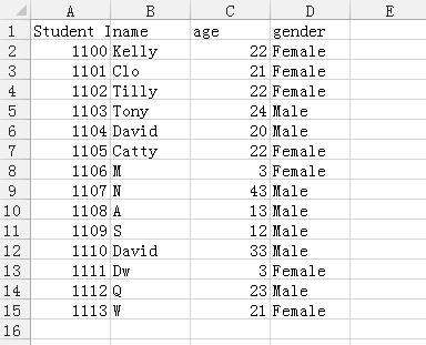
1 2 3 4 5 6 7 8 9 10 11 12 13 14 15 16 17 18 19 20 21 22 23 24 25 26 27 28 29 | In [33]: import pandas as pdIn [34]: data = pd.read_csv('student.csv')In [35]: print(data) Student ID name age gender0 1100 Kelly 22 Female1 1101 Clo 21 Female2 1102 Tilly 22 Female3 1103 Tony 24 Male4 1104 David 20 Male5 1105 Catty 22 Female6 1106 M 3 Female7 1107 N 43 Male8 1108 A 13 Male9 1109 S 12 Male10 1110 David 33 Male11 1111 Dw 3 Female12 1112 Q 23 Male13 1113 W 21 FemaleIn [36]: print(type(data))<class 'pandas.core.frame.DataFrame'>In [37]: data.to_pickle('student.pickle')In [38]: data.to_json('student.json')In [39]: |
更多IO Tools参考:官方介绍
Pandas concat合并
1 2 3 4 5 6 7 8 9 10 11 12 13 14 15 16 17 18 19 20 21 22 23 24 25 26 27 28 29 30 31 32 33 34 35 36 37 38 39 40 41 42 43 44 45 46 47 48 49 50 51 52 53 54 55 56 57 58 59 60 61 62 63 64 65 66 67 68 69 70 71 72 73 74 75 76 77 78 79 80 81 82 83 84 85 86 87 88 89 90 91 92 93 94 95 96 97 98 99 100 101 102 103 104 105 106 107 108 109 110 111 112 113 114 115 116 117 118 119 120 121 122 123 124 125 126 127 128 129 130 131 132 133 134 135 136 137 138 139 140 141 142 143 144 145 146 147 148 149 150 151 152 153 154 155 156 157 158 159 160 161 162 163 164 165 166 167 168 169 170 171 172 173 174 175 176 177 178 179 180 181 182 183 184 185 186 187 188 189 190 191 192 193 194 195 196 197 198 199 200 201 202 203 204 205 206 207 208 209 210 211 212 213 214 215 216 217 218 219 220 221 | # pandas 合并# concatenatingIn [40]: import numpy as npIn [41]: import pandas as pdIn [42]: df1 = pd.DataFrame(np.ones((3,4))*0, columns=['a','b','c','d'])In [43]: df2 = pd.DataFrame(np.ones((3,4))*1, columns=['a','b','c','d'])In [44]: df3 = pd.DataFrame(np.ones((3,4))*2, columns=['a','b','c','d'])In [45]: print(df1) a b c d0 0.0 0.0 0.0 0.01 0.0 0.0 0.0 0.02 0.0 0.0 0.0 0.0In [46]: print(df2) a b c d0 1.0 1.0 1.0 1.01 1.0 1.0 1.0 1.02 1.0 1.0 1.0 1.0In [47]: print(df3) a b c d0 2.0 2.0 2.0 2.01 2.0 2.0 2.0 2.02 2.0 2.0 2.0 2.0In [48]: result = pd.concat([df1,df2,df3],axis=0) # vertical 垂直合并In [49]: print(result) a b c d0 0.0 0.0 0.0 0.01 0.0 0.0 0.0 0.02 0.0 0.0 0.0 0.00 1.0 1.0 1.0 1.01 1.0 1.0 1.0 1.02 1.0 1.0 1.0 1.00 2.0 2.0 2.0 2.01 2.0 2.0 2.0 2.02 2.0 2.0 2.0 2.0In [50]: In [50]: result = pd.concat([df1,df2,df3],axis=0,ignore_index=True) # 序号重新排列In [51]: print(result) a b c d0 0.0 0.0 0.0 0.01 0.0 0.0 0.0 0.02 0.0 0.0 0.0 0.03 1.0 1.0 1.0 1.04 1.0 1.0 1.0 1.05 1.0 1.0 1.0 1.06 2.0 2.0 2.0 2.07 2.0 2.0 2.0 2.08 2.0 2.0 2.0 2.0In [52]:# join合并 ['inner','outer']In [63]: df1 = pd.DataFrame(np.ones((3,4))*0, columns=['a','b','c','d'],index=[1,2,3])In [64]: df2 = pd.DataFrame(np.ones((3,4))*1, columns=['b','c','d','e'],index=[2,3,4])In [65]: print(df1) a b c d1 0.0 0.0 0.0 0.02 0.0 0.0 0.0 0.03 0.0 0.0 0.0 0.0In [66]: print(df2) b c d e2 1.0 1.0 1.0 1.03 1.0 1.0 1.0 1.04 1.0 1.0 1.0 1.0In [67]: In [67]: result = pd.concat([df1,df2]) # 即 pd.concat([df1,df2],join='outer') , 默认就是outer模式/usr/local/anaconda2/bin/ipython2:1: FutureWarning: Sorting because non-concatenation axis is not aligned. A future versionof pandas will change to not sort by default.To accept the future behavior, pass 'sort=True'.To retain the current behavior and silence the warning, pass sort=False #!/usr/local/anaconda2/bin/pythonIn [68]: In [68]: print(result) a b c d e1 0.0 0.0 0.0 0.0 NaN2 0.0 0.0 0.0 0.0 NaN3 0.0 0.0 0.0 0.0 NaN2 NaN 1.0 1.0 1.0 1.03 NaN 1.0 1.0 1.0 1.04 NaN 1.0 1.0 1.0 1.0In [69]:In [70]: result = pd.concat([df1,df2],join='inner') # inner模式In [71]: print(result) b c d1 0.0 0.0 0.02 0.0 0.0 0.03 0.0 0.0 0.02 1.0 1.0 1.03 1.0 1.0 1.04 1.0 1.0 1.0In [72]: In [72]: result = pd.concat([df1,df2],join='inner',ignore_index=True)In [73]: print(result) b c d0 0.0 0.0 0.01 0.0 0.0 0.02 0.0 0.0 0.03 1.0 1.0 1.04 1.0 1.0 1.05 1.0 1.0 1.0In [74]: # join_axes合并In [78]: res = pd.concat([df1, df2], axis=1)In [79]: print(res) a b c d b c d e1 0.0 0.0 0.0 0.0 NaN NaN NaN NaN2 0.0 0.0 0.0 0.0 1.0 1.0 1.0 1.03 0.0 0.0 0.0 0.0 1.0 1.0 1.0 1.04 NaN NaN NaN NaN 1.0 1.0 1.0 1.0In [80]: In [74]: df1 = pd.DataFrame(np.ones((3,4))*0, columns=['a','b','c','d'],index=[1,2,3])In [75]: df2 = pd.DataFrame(np.ones((3,4))*1, columns=['b','c','d','e'],index=[2,3,4])In [76]: res = pd.concat([df1, df2], axis=1, join_axes=[df1.index])In [77]: print(res) a b c d b c d e1 0.0 0.0 0.0 0.0 NaN NaN NaN NaN2 0.0 0.0 0.0 0.0 1.0 1.0 1.0 1.03 0.0 0.0 0.0 0.0 1.0 1.0 1.0 1.0In [78]: In [80]: res = pd.concat([df1, df2], axis=1, join_axes=[df2.index])In [81]: print(res) a b c d b c d e2 0.0 0.0 0.0 0.0 1.0 1.0 1.0 1.03 0.0 0.0 0.0 0.0 1.0 1.0 1.0 1.04 NaN NaN NaN NaN 1.0 1.0 1.0 1.0In [82]: # append合并In [87]: df1 = pd.DataFrame(np.ones((3,4))*0, columns=['a','b','c','d'])In [88]: df2 = pd.DataFrame(np.ones((3,4))*1, columns=['a','b','c','d'])In [89]: df1.append(df2,ignore_index=True)Out[89]: a b c d0 0.0 0.0 0.0 0.01 0.0 0.0 0.0 0.02 0.0 0.0 0.0 0.03 1.0 1.0 1.0 1.04 1.0 1.0 1.0 1.05 1.0 1.0 1.0 1.0In [90]: df3 = pd.DataFrame(np.ones((3,4))*1, columns=['a','b','c','d'])In [91]: df1.append([df2,df3],ignore_index=True)Out[91]: a b c d0 0.0 0.0 0.0 0.01 0.0 0.0 0.0 0.02 0.0 0.0 0.0 0.03 1.0 1.0 1.0 1.04 1.0 1.0 1.0 1.05 1.0 1.0 1.0 1.06 1.0 1.0 1.0 1.07 1.0 1.0 1.0 1.08 1.0 1.0 1.0 1.0In [92]: # 添加一行数据到DataFrameIn [92]: df1 = pd.DataFrame(np.ones((3,4))*0, columns=['a','b','c','d'])In [93]: s1 = pd.Series([1,2,3,4], index=['a','b','c','d'])In [94]: res = df1.append(s1,ignore_index=True)In [95]: print(res) a b c d0 0.0 0.0 0.0 0.01 0.0 0.0 0.0 0.02 0.0 0.0 0.0 0.03 1.0 2.0 3.0 4.0In [96]: |
Pandas merge合并
1 2 3 4 5 6 7 8 9 10 11 12 13 14 15 16 17 18 19 20 21 22 23 24 25 26 27 28 29 30 31 32 33 34 35 36 37 38 39 40 41 42 43 44 45 46 47 48 49 50 51 52 53 54 55 56 57 58 59 60 61 62 63 64 65 66 67 68 69 70 71 72 73 74 75 76 77 78 79 80 81 82 83 84 85 86 87 88 89 90 91 92 93 94 95 96 97 98 99 100 101 102 103 104 105 106 107 108 109 110 111 112 113 114 115 116 117 118 119 120 121 122 123 124 125 126 127 128 129 130 131 132 133 134 135 136 137 138 139 140 141 142 143 144 145 146 147 148 149 150 151 152 153 154 155 156 157 158 159 160 161 162 163 164 165 166 167 168 169 170 171 172 173 174 175 176 177 178 179 180 181 182 183 184 185 186 187 188 189 190 191 192 193 194 195 196 197 198 199 200 201 202 203 204 205 206 207 208 209 210 211 212 213 214 215 216 217 218 219 220 221 222 223 224 225 226 227 228 229 230 231 232 233 234 235 236 237 238 239 240 241 242 243 244 245 246 247 248 | # merge合并In [99]: import pandas as pdIn [100]: left = pd.DataFrame({'key': ['K0', 'K1', 'K2', 'K3'], ...: 'A': ['A0', 'A1', 'A2', 'A3'], ...: 'B': ['B0', 'B1', 'B2', 'B3']})In [101]: right = pd.DataFrame({'key': ['K0', 'K1', 'K2', 'K3'], ...: 'C': ['C0', 'C1', 'C2', 'C3'], ...: 'D': ['D0', 'D1', 'D2', 'D3']})In [102]: In [102]: print(left) A B key0 A0 B0 K01 A1 B1 K12 A2 B2 K23 A3 B3 K3In [103]: print(right) C D key0 C0 D0 K01 C1 D1 K12 C2 D2 K23 C3 D3 K3In [104]: In [104]: res = pd.merge(left,right,on='key')In [105]: print(res) A B key C D0 A0 B0 K0 C0 D01 A1 B1 K1 C1 D12 A2 B2 K2 C2 D23 A3 B3 K3 C3 D3In [106]: # consider two keysIn [106]: left = pd.DataFrame({'key1': ['K0', 'K0', 'K1', 'K2'], ...: 'key2': ['K0', 'K1', 'K0', 'K1'], ...: 'A': ['A0', 'A1', 'A2', 'A3'], ...: 'B': ['B0', 'B1', 'B2', 'B3']})In [107]: right = pd.DataFrame({'key1': ['K0', 'K1', 'K1', 'K2'], ...: 'key2': ['K0', 'K0', 'K0', 'K0'], ...: 'C': ['C0', 'C1', 'C2', 'C3'], ...: 'D': ['D0', 'D1', 'D2', 'D3']})In [108]: print(left) A B key1 key20 A0 B0 K0 K01 A1 B1 K0 K12 A2 B2 K1 K03 A3 B3 K2 K1In [109]: print(right) C D key1 key20 C0 D0 K0 K01 C1 D1 K1 K02 C2 D2 K1 K03 C3 D3 K2 K0In [110]: res = pd.merge(left,right,on=['key1','key2'])In [111]: print(res) A B key1 key2 C D0 A0 B0 K0 K0 C0 D01 A2 B2 K1 K0 C1 D12 A2 B2 K1 K0 C2 D2# how={'left','right','inner','outer'}In [112]: res = pd.merge(left,right,on=['key1','key2'],how='inner') # 默认就是inner模式In [113]: print(res) A B key1 key2 C D0 A0 B0 K0 K0 C0 D01 A2 B2 K1 K0 C1 D12 A2 B2 K1 K0 C2 D2In [114]: res = pd.merge(left,right,on=['key1','key2'],how='outer')In [115]: print(res) A B key1 key2 C D0 A0 B0 K0 K0 C0 D01 A1 B1 K0 K1 NaN NaN2 A2 B2 K1 K0 C1 D13 A2 B2 K1 K0 C2 D24 A3 B3 K2 K1 NaN NaN5 NaN NaN K2 K0 C3 D3In [116]: In [116]: res = pd.merge(left,right,on=['key1','key2'],how='left')In [117]: print(res) A B key1 key2 C D0 A0 B0 K0 K0 C0 D01 A1 B1 K0 K1 NaN NaN2 A2 B2 K1 K0 C1 D13 A2 B2 K1 K0 C2 D24 A3 B3 K2 K1 NaN NaNIn [118]: res = pd.merge(left,right,on=['key1','key2'],how='right')In [119]: print(res) A B key1 key2 C D0 A0 B0 K0 K0 C0 D01 A2 B2 K1 K0 C1 D12 A2 B2 K1 K0 C2 D23 NaN NaN K2 K0 C3 D3In [120]: # indicatorIn [121]: df1 = pd.DataFrame({'col1':[0,1], 'col_left':['a','b']})In [122]: df2 = pd.DataFrame({'col1':[1,2,2],'col_right':[2,2,2]})In [123]: print(df1) col1 col_left0 0 a1 1 bIn [124]: print(df2) col1 col_right0 1 21 2 22 2 2In [125]: res = pd.merge(df1, df2, on='col1', how='outer', indicator=True) # 给一个提示In [126]: print(res) col1 col_left col_right _merge0 0 a NaN left_only1 1 b 2.0 both2 2 NaN 2.0 right_only3 2 NaN 2.0 right_onlyIn [127]:In [129]: res = pd.merge(df1, df2, on='col1', how='outer', indicator='indicator_column') # 指定提示的列名In [130]: print(res) col1 col_left col_right indicator_column0 0 a NaN left_only1 1 b 2.0 both2 2 NaN 2.0 right_only3 2 NaN 2.0 right_onlyIn [131]: In [127]: res = pd.merge(df1, df2, on='col1', how='outer', indicator=False)In [128]: print(res) col1 col_left col_right0 0 a NaN1 1 b 2.02 2 NaN 2.03 2 NaN 2.0In [129]: In [131]: left = pd.DataFrame({'A': ['A0', 'A1', 'A2'], ...: 'B': ['B0', 'B1', 'B2']}, ...: index=['K0', 'K1', 'K2'])In [132]: right = pd.DataFrame({'C': ['C0', 'C2', 'C3'], ...: 'D': ['D0', 'D2', 'D3']}, ...: index=['K0', 'K2', 'K3'])In [133]: print(left) A BK0 A0 B0K1 A1 B1K2 A2 B2In [134]: print(right) C DK0 C0 D0K2 C2 D2K3 C3 D3In [135]: res = pd.merge(left, right, left_index=True, right_index=True, how='outer')In [136]: print(res) A B C DK0 A0 B0 C0 D0K1 A1 B1 NaN NaNK2 A2 B2 C2 D2K3 NaN NaN C3 D3In [137]: res = pd.merge(left, right, left_index=True, right_index=True, how='inner')In [138]: print(res) A B C DK0 A0 B0 C0 D0K2 A2 B2 C2 D2In [139]: # handle overlappingIn [139]: boys = pd.DataFrame({'k': ['K0', 'K1', 'K2'], 'age': [1, 2, 3]})In [140]: girls = pd.DataFrame({'k': ['K0', 'K0', 'K3'], 'age': [4, 5, 6]})In [141]: print(boys) age k0 1 K01 2 K12 3 K2In [142]: print(girls) age k0 4 K01 5 K02 6 K3In [143]: res = pd.merge(boys, girls, on='k', suffixes=['_boy', '_girl'], how='inner')In [144]: print(res) age_boy k age_girl0 1 K0 41 1 K0 5In [145]: res = pd.merge(boys, girls, on='k', suffixes=['_boy', '_girl'], how='outer')In [146]: print(res) age_boy k age_girl0 1.0 K0 4.01 1.0 K0 5.02 2.0 K1 NaN3 3.0 K2 NaN4 NaN K3 6.0In [147]: |
Pandas Moving Window Functions
Pandas plot可视化
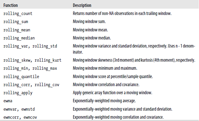
1 2 3 4 5 6 7 8 9 10 11 12 13 14 | #!/usr/bin/python2.7import numpy as npimport pandas as pdimport matplotlib.pyplot as plt# Seriesdata = pd.Series(np.random.randn(1000),index=np.arange(1000))data = data.cumsum()data.plot()plt.show() |
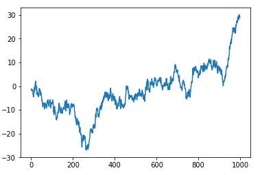
1 2 3 4 5 6 7 8 9 10 11 12 13 14 15 | #!/usr/bin/python2.7import numpy as npimport pandas as pdimport matplotlib.pyplot as plt# DataFramedata = pd.DataFrame(np.random.randn(1000,4),\ index=np.arange(1000), \ columns=list("ABCD"))data = data.cumsum()# print(data.head(6))data.plot()plt.show() |
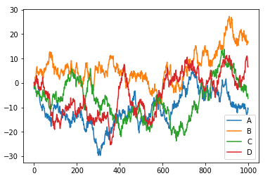
1 2 3 4 5 6 7 8 9 10 11 12 13 14 15 16 17 18 | #!/usr/bin/python2.7import numpy as npimport pandas as pdimport matplotlib.pyplot as plt# DataFramedata = pd.DataFrame(np.random.randn(1000,4),\ index=np.arange(1000), \ columns=list("ABCD"))data = data.cumsum()# print(data.head(6))# plot method:# 'bar','hist','box','kde','aera','scatter','pie','hexbin'...ax = data.plot.scatter(x='A',y='B',color='DarkBlue',label='Class AB')data.plot.scatter(x='A',y='C',color='DarkGreen',label='Class AC',ax=ax)plt.show() |
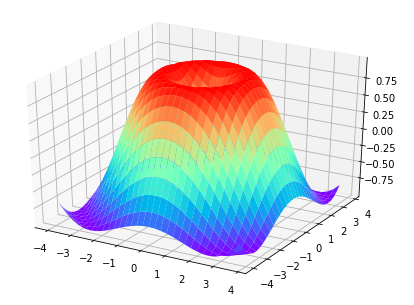
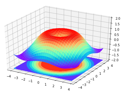
补充:Matplotlib 3D图像
1 2 3 4 5 6 7 8 9 10 11 12 13 14 15 16 17 18 19 20 21 | #!/usr/bin/python2.7import numpy as npimport matplotlib.pyplot as pltfrom mpl_toolkits.mplot3d import Axes3Dfig = plt.figure()ax = Axes3D(fig)# X,Y valueX = np.arange(-4,4,0.25)Y = np.arange(-4,4,0.25)X,Y = np.meshgrid(X,Y)R = np.sqrt(X**2+Y**2)# height valueZ = np.sin(R)ax.plot_surface(X,Y,Z,rstride=1,cstride=1,cmap=plt.get_cmap('rainbow'))plt.show() |
1 2 3 4 5 6 7 8 9 10 11 12 13 14 15 16 17 18 19 20 21 22 23 24 25 | #!/usr/bin/python2.7import numpy as npimport matplotlib.pyplot as pltfrom mpl_toolkits.mplot3d import Axes3Dfig = plt.figure()ax = Axes3D(fig)# X,Y valueX = np.arange(-4,4,0.25)Y = np.arange(-4,4,0.25)X,Y = np.meshgrid(X,Y)R = np.sqrt(X**2+Y**2)# height valueZ = np.sin(R)ax.plot_surface(X,Y,Z,rstride=1,cstride=1,cmap=plt.get_cmap('rainbow'))ax.contourf(X,Y,Z,zdir='z',offset=-2,cmap='rainbow') # 增加等高线ax.set_zlim(-2,2)plt.show() |
参考:https://github.com/MorvanZhou
参考:https://morvanzhou.github.io/tutorials/
作者:Standby — 一生热爱名山大川、草原沙漠,还有我们小郭宝贝!
出处:http://www.cnblogs.com/standby/
本文版权归作者和博客园共有,欢迎转载,但未经作者同意必须保留此段声明,且在文章页面明显位置给出原文连接,否则保留追究法律责任的权利。
出处:http://www.cnblogs.com/standby/
本文版权归作者和博客园共有,欢迎转载,但未经作者同意必须保留此段声明,且在文章页面明显位置给出原文连接,否则保留追究法律责任的权利。


【推荐】国内首个AI IDE,深度理解中文开发场景,立即下载体验Trae
【推荐】Flutter适配HarmonyOS 5知识地图,实战解析+高频避坑指南
【推荐】凌霞软件回馈社区,携手博客园推出1Panel与Halo联合会员
【推荐】轻量又高性能的 SSH 工具 IShell:AI 加持,快人一步
· 领域驱动设计实战:聚合根设计与领域模型实现
· 突破Excel百万数据导出瓶颈:全链路优化实战指南
· 如何把ASP.NET Core WebApi打造成Mcp Server
· Linux系列:如何用perf跟踪.NET程序的mmap泄露
· 日常问题排查-空闲一段时间再请求就超时
· .NET周刊【5月第1期 2025-05-04】
· Python 3.14 新特性盘点,更新了些什么?
· 聊聊 ruoyi-vue ,ruoyi-vue-plus ,ruoyi-vue-pro 谁才是真正的
· 物联网之对接MQTT最佳实践
· Redis 连接池耗尽的一次异常定位
2017-08-12 前端基础之JQuery